Every telescope or telephoto lens has its “magic” f/number: that is, the ratio between its focal length and aperture. Although we don’t go deeper into the matter as it’s not within the scope of this article, it’s worth mentioning that the higher the f/ratio, the longer the exposure time required to yield a given picture density (i.e. how much detail we want to record).
Each telephoto lens is normally used with the camera body it was built for, so that when we adjust the lens’ aperture wheel, we’re pretty much sure our shot will be taken with that very focal ratio we selected by rotating the wheel. On the other hand, telescopes have no aperture wheel and are rated at a given focal length (or f/ratio); however, this can vary quite widely according to what we put in the optical train between the main lens/mirror and the imaging sensor (be it film or digital). Accessories such as adapters, rings, focal reducers, off-axis guiders, tele-extenders, barlows, etc. can yield an actual equivalent focal ratio which can be very different from the original one. This is especially true of such telescopes as SCTs, whose optical configuration allows for a huge backfocus thereby enabling the use of a host of optical and mechanical add-ons.
In this article I describe a way to precisely figure out the equivalent focal ratio an image was shot at. It applies to all kinds of optics and imaging sensors: however, there are some (lower) focal length limits with the source of the images used as a reference in our calculations, and not with the method per se. The main steps of the “algorithm” can be summarized as follows: I take my picture and compare it to a reference one whose scale and dimensions are precisely known a priori. I then can calculate the angular field covered by my picture and finally the equivalent focal ratio.
How do I get my reference image? Needless to say, the answer comes from the Internet: the STScI’s (Space Telescope Science Institute) Digital Sky survey is a huge image archive covering most, if not all, of the celestial dome with scales down to 1.0 arcsecs/pixel. The DSS can be found here, where an on-line form can be filled out to get the desired image. We can proceed as follows:
- We should know the equatorial coordinates (i.e RA, DEC epoch J2000) of the center of our frame. If we don’t, we can derive them from a star atlas or we can even try to find them by feeding in the name of our target (e.g. a Messier or NGC object) into the fields in the upper part of the form. If we get lucky enough, the coordinate field will be automatically filled in as soon as the response comes from the server.
- We now can retrieve the image centered on the given coordinates as follows:
- Choose the data source (“Retrieve from…” item). They all are more or less the same for our measurement purposes; however, since they are generally taken in other spectral bands than visible light, the layout and brightness of the reference stars could differ from our image.
- Enter coordinates (either known or calculated in step 1)
- Enter height (Declination) and width (RA). Maximum possible values are 60′ (i.e. 1 degree) in both directions.
- Choose file format: GIF is better for our purpose because of useability with common programs like Photoshop. FITS images are more suitable if image processing is required for their greater detail quality and dynamic range. Be aware, though, that a 1-square-degree GIF can be really hefty (about 5-8 Mb).
- Choose “no HST field of view overlay”
- Download and save reference image.
- Later on, we can open both our original (or “unknown”) picture and reference image in Photoshop. We then spot a pair of stars in both images which are enough apart to give a good measurement: say, at least one third of our original shot, and we measure their distance in pixels for both images.
- Since the angular scale for our reference image is well known or can be easily derived, we can figure out the image pixel scale for our original picture and finally its angular dimensions.
- Finally, computing our rig’s equivalent focal ratio is really a breeze.
The math is quite straightforward. Let
- α a be the real angular separation between two reference stars A and B
 be the scales (in arcsecs / pixel) of our test and reference image. The latter is known, while the former has to be calculated.
 be the separations in pixels between the centers of stars A and B for our test and reference image respectively.
Since α is the same no matter which image we are looking at, the following applies:
When the scale for our test image is known, we can easily calculate its angular dimensions from its width and height in pixels through the following:
Where d is the actual frame size used as a reference (e.g. the width of the slide in millimeters), F the equivalent focal length of our optical train; both d and F must be in the same units; the 57.3 constant comes from the angle-to-radians conversion (i.e. 180 / PI). We then divide F by the aperture of our telescope and get the final equivalent f/ratio.
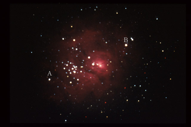
Well, let’s now get to a practical example to see what it is all about. As a test, I’ve picked out a 20-minute picture of M8 (Lagoon Nebula) I took on March 31st, 2001 at the prime focus of a 12″ Meade LX200 SCT. The image looks way out of focus and suffers from severe vignetting, since I used my Lumicon Cassegrain Easy Guider instead of the Giant Easy Guider which fits 10″ and larger SCTs. Nevertheless, this is a nice test because the off-axis guider has a focal reducer, which yields different focal ratios depending on its position in the guider’s main body. Our aim is now to figure out the actual f/ratio M8 was shot at. Here is our test image:
And here is our reference image (courtesy STScI):
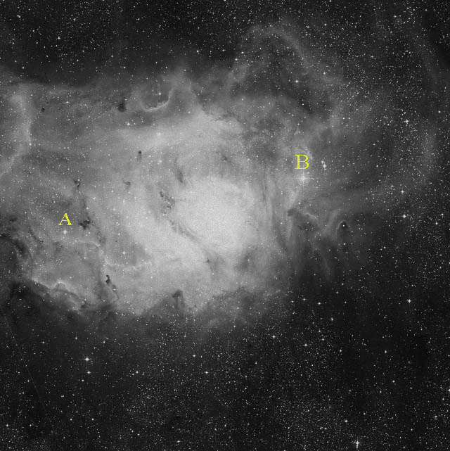
Both images were scaled down to more manageable sizes (i.e. reduced to about 1/6) for web publication, then we marked the reference stars A and B in both of them. In the reference image stars A and B are 1934 pixels apart, while in our test image their distance is 1710 pixels. Since the scale for our reference is 1.0 arcsec/pixel according to the DSS site itself, AB is 1934 arcsecs across; therefore, according to equation 1 our test image has a scale of 1934/1710 = 1.131 arcsec/pixel.
The reference image was scanned at 2700 dpi, so that its width (36 mm) is 3827 pixels: at 1.131 arcsecs/pixels, this yields 4328 arcsecs or 1.2022 ~ 1.20 degrees. As per equation 2, the equivalent focal length turns out to be (57.3 x 36) / 1.20 = 1719 mm. Since the ‘scope aperture was 12 inches or 305 mm, we find the f/ratio to be 1719 / 305, or about f/5.64, which is a very reasonable figure.
This method only needs a few measurements and simple calculations, and in my humble opinion it’s already quite reliable “as is”; however, there are other ways for further improving our precision, e.g. by averaging our distance over more than one pair of stars. The only flaw I see is with our reference image source, whose size is limited to one square degree: we therefore can’t get accurate measurements of widefield images covering several degrees of sky. The only solution to this problem would be finding larger images, but then we should factor in the mathematical approximation implied in equation 2: for very small angles (say < 2 degs), tan (angle) ~ angle, where angle is expressed in radians.
One final note: this procedure is equally suited for digital (that is, taken with a CCD or a DSLR camera) and analog (i.e. shot with film and digitized through a scanner) images.